Graph Algorithms

This section will guide you through using graph algorithms within the Timbr environment. You'll discover the range of available graph algorithms, learn how to construct SQL queries for these algorithms, and understand the transformation of these queries into graph structures. Additionally, you'll explore the application of various graph algorithms on these structures, equipping you with the knowledge to analyze complex data effectively.

Supported Algorithms

The currently supported graph algorithms can be found in the gtimbr schema. They can be run on CPU or GPU (if supported by the infrastructure)

The currently supported graph algorithms are:

Centrality

betweenness centrality - Compute the shortest-path betweenness centrality for nodes. More information (Timbr sets a default threshold of 0.25, considering only nodes with centrality scores above this value to optimize analysis and performance)
katz - Compute the Katz centrality for the nodes of the graph G. More information (Timbr sets a default threshold of 0.25, considering only nodes with centrality scores above this value to optimize analysis and performance)

Classification

node classification - Node classification by Harmonic function. More information
pagerank - Link classification. Returns the PageRank of the nodes in the graph. More information

Community Detection

louvain - Find the best partition of a graph using the Louvain Community Detection Algorithm. Louvain Community Detection Algorithm is a simple method to extract the community structure of a network. This is a heuristic method based on modularity optimization.More information

Components

strongly cc - Generate nodes in strongly connected components of graph. More information
weakly cc - Generate weakly connected components of graph. More information

Cores

core number - Returns the core number for each vertex. More information

Cycles

cycle basis - Returns a list of cycles which form a basis for cycles of G. More information
simple cycles - Find simple cycles (elementary circuits) of a graph. More information
recursive simple cycles - Find simple cycles (elementary circuits) of a directed graph. More information

Link Prediction

common neighbor centrality - Compute the Common Neighbor and Centrality based Parameterized Algorithm(CCPA) score of all node pairs in ebunch. More information (A default threshold of 0.25 is set in Timbr to consider only connections with a minimum similarity of 0.25)
jaccard - Compute the Jaccard coefficient of all node pairs in ebunch. More information (A default threshold of 0.25 is set in Timbr to consider only connections with a minimum similarity of 0.25)
jaccard fuzzy - Compute the Jaccard coefficient of all node pairs matched by fuzzy matching in ebunch. More information (A default threshold of 0.25 is set in Timbr to consider only connections with a minimum similarity of 0.25)
overlap - Compute the Overlap Coefficient between each pair of vertices connected by an edge, or between arbitrary pairs of vertices specified by the user. More information

In addition to the supported algorithms above, Timbr can support any graph algorithm that is currently supported by:

CPU based NetworkX or cuGraph
Graph based cuGraph

Build a query for the graph algorithm

Structure of the Query in Timbr:

The query begins with a SELECT statement, identifying the columns to be included. In Timbr, these columns are interpreted as nodes or elements of the graph, which are essential for the algorithm's processing.

First Column as the ID:

The first column following the SELECT is crucial, as it serves as the ID returned from the algorithm. This column is the primary identifier for the elements within the graph, guiding how the algorithm processes and understands the graph's structure.

For example, in a query such as:

SELECT customer_id, product_id FROM dtimbr.customer

customer_id that appears first after the SELECT will be the ID returned from the algorithm and will serve as the primary identifier for the elements within the graph. If product_id appeared first, then it would assume the role of the primary identifier.

This holds true for all algorithms, whether it be the Louvain Community Detection algorithm, the Jaccard Similarity algorithm, or any other algorithm.

Handling Same IDs in Different Result Columns:

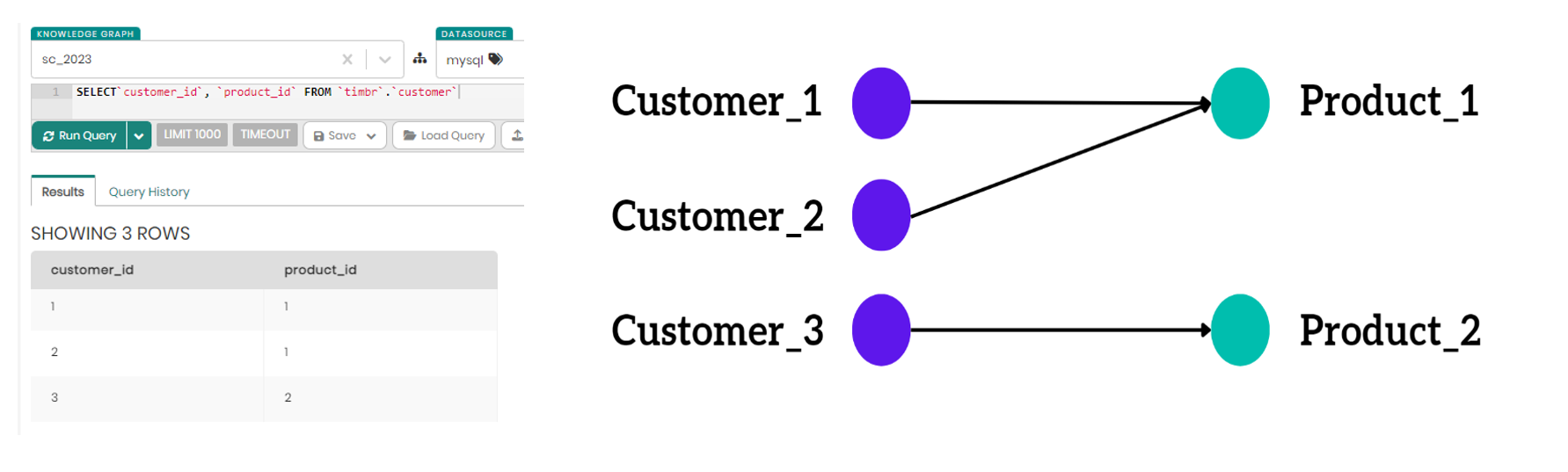
• When identical IDs are found in different columns, Timbr adds a prefix to each ID behind the scenes to maintain its uniqueness. This differentiation is key to ensuring each identifier in the graph is distinct. For example, in the query results for:

SELECT customer_id, product_id FROM dtimbr.customer

If both customer_id and product_id have identical IDs of 1, Timbr will prefix each ID (e.g., customer_1, product_1) to maintain their uniqueness.

prefix

• In situations where two columns are intended to have the same ID, an alias is crucial not just for alignment but to explicitly define the relationship between the columns and prevent ambiguity. Therefore, for the query:

SELECT product_id, related_product_id FROM dtimbr.customer

We must add an alias to related_product_id to align it with the primary identifier product_id, resulting in the query:

SELECT product_id, related_product_id as related_product_id.product_id FROM dtimbr.customer

The alias related_product_id.product_id signifies its direct relationship to the primary identifier product_id.

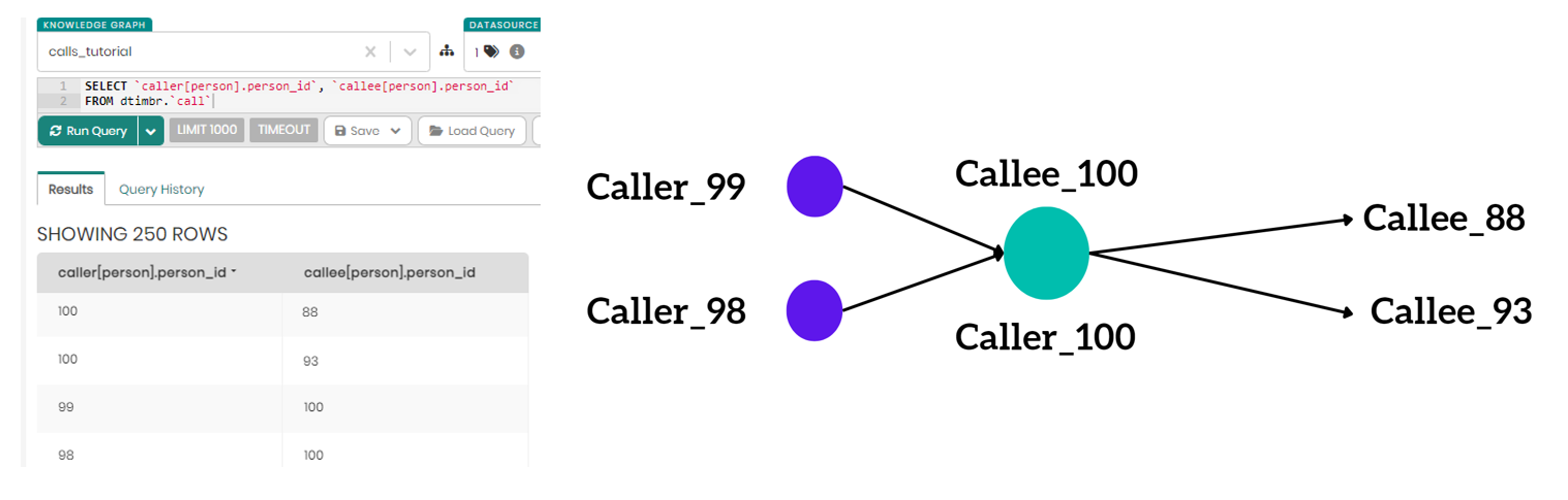
There are scenarios where an alias might not be necessary, as in the query:

SELECT caller[person].person_id, callee[person].person_id FROM dtimbr.call

where the second column naturally aligns with the first, as both end with .person_id. Here, the results would clearly indicate, for example as shown below, a caller with the identifier 100 appearing in both columns, identified by Timbr as the same entity acting as both caller and callee.

alias

Query the graph algorithm

To query a graph algorithm, all that is needed is to query the gtimbr schema for a supported graph algorithm specified above.

Each graph algorithm may require a different amount of inputs in order to run correctly.
You can see the number of input variables required by querying the metadata of the graph algorithm selected in the gtimbr schema.
The input variable of the graph on which to perform the graph algorithm is a Timbr SQL query that is passed as a parameter to the graph algorithm you want to run.
The output of running a graph algorithm may have a different number of columns depending on the graph algorithm that was executed.

Required information for querying a graph algorithm (the curly brackets {} should not be an input, they are used only as a variable substitution):

{graph_algorithm} - The name of the graph algorithm you want to run
{timbr_sql_query} - The SQL query that makes up the graph on which the graph algorithm is executed.

SELECT * from gtimbr.{graph_algorithm}(
{timbr_sql_query}
)

Example using the Louvain graph algorithm

SELECT * from gtimbr.louvain(
  select `organization_id`, `made_investment[funding_round].organization_id`
  from dtimbr.financial_organization
  limit 1000
)

Add Query Parameters

Query parameters are pivotal tools that allow you to fine-tune how algorithms interpret and analyze your data.

Graph Projection

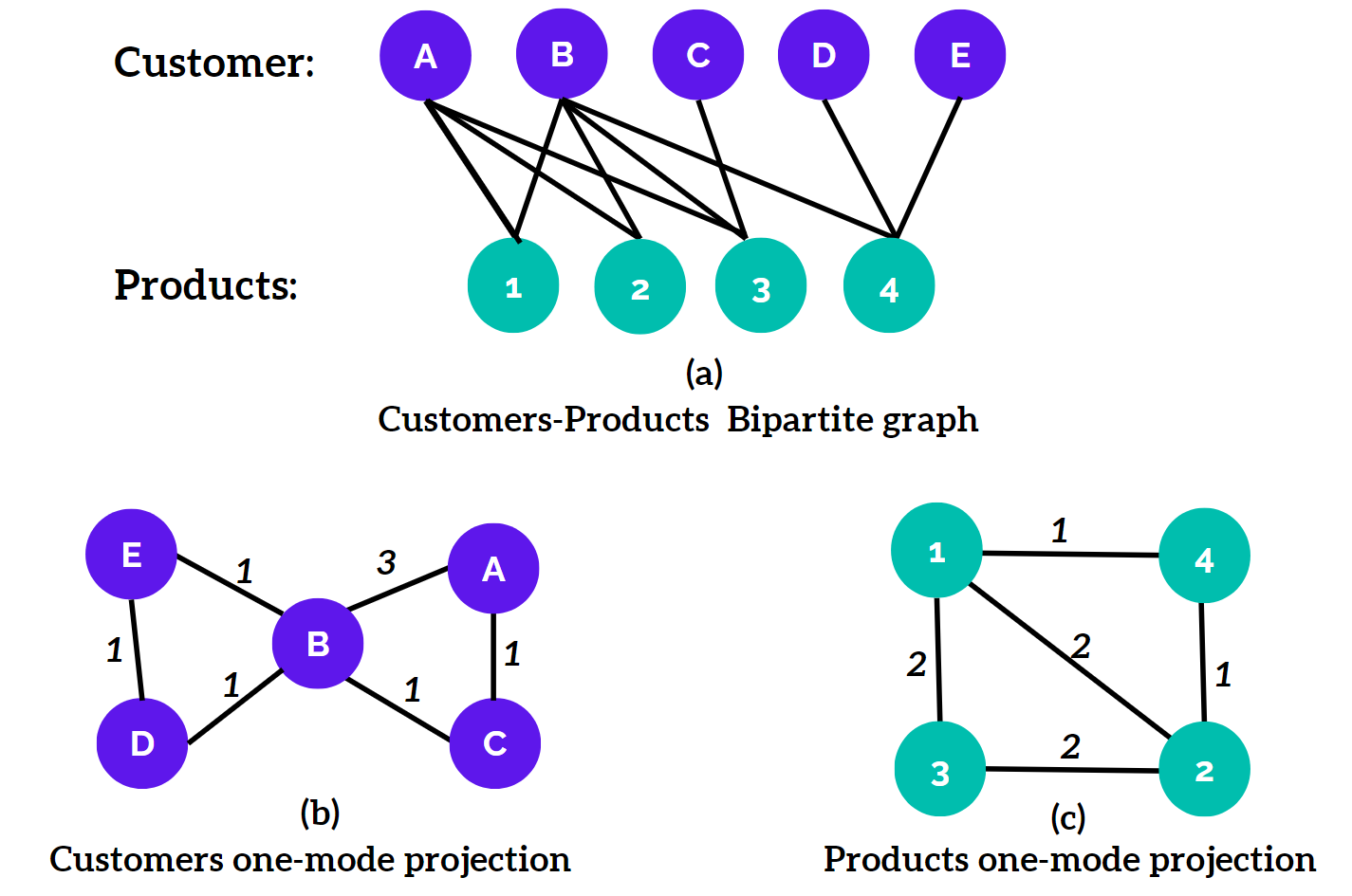
Graph projection is a process where a graph is transformed or 'projected' into a simpler version, often focusing on a subset of its elements.

Not all graph algorithms inherently understand how to process different types of nodes in a graph, for example, customer_id, product_id and location_id. By default, Timbr automatically selects the node types that the algorithm is compatible with. However, the graph projection parameter empowers users to override this default behavior. When set to 'true', it instructs the algorithm to consider all types of nodes in the data, potentially leading to a more complex graph structure. Conversely, setting it to 'false' maintains the default behavior, where the algorithm focuses only on the node types it can naturally handle. This flexibility allows users to tailor the graph structure to their specific analytical needs.

In addition, the "weighted_projected_graph" function is used by Timbr to project a bipartite network onto one of its node sets, with edge weights reflecting the number of shared neighbors or their ratio. This function is crucial when dealing with complex data where relationships between different node types (like customer_id, product_id, location_id) are essential. By integrating "weighted_projected_graph" with the "graph_projection" parameter, Timbr can effectively handle diverse node types in a graph, enhancing the algorithm's ability to deal with multi-dimensional data structures.

graph_projection

Required information for adding the graph projection parameter in a graph algorithm query(the curly brackets {} should not be an input, they are used only as a variable substitution):

{graph_algorithm} - The name of the graph algorithm you want to run
{timbr_sql_query} - The SQL query that makes up the graph on which the graph algorithm is executed.

SELECT * from gtimbr.{graph_algorithm}( 
    ({timbr_sql_query}), 
    graph_projection ='false'/'true'
    )

Example using the graph projection parameter

SELECT * from gtimbr.louvain(
    (SELECT customer_id, product_id),
    graph_projection = 'false'
)

Threshold

The threshold parameter refers to a cut-off value or criterion used to filter or determine the inclusion of elements in the analysis. For example, in the context of network analysis, it might be used to define the minimum level of interaction or connection strength required for an edge to be considered significant and included in the graph. This parameter is crucial for refining the graph to focus on more relevant or stronger connections, thereby enhancing the meaningfulness and clarity of the analysis.

The threshold parameter plays a pivotal role in graph algorithms within Timbr. It acts as a filter to determine the minimum level of significance for relationships in the graph. For instance, in algorithms like Jaccard, a default threshold of 0.25 is set to consider only connections with a minimum similarity of 0.25. Similarly, in betweenness centrality, nodes with centrality scores below 0.25 are filtered out. This threshold not only focuses the analysis on more meaningful data but also enhances computing efficiency by limiting the results processed, balancing detailed analysis with performance optimization.

In Addition, Timbr incorporates a built-in default, returning only the top 3 similarities in certain algorithms to manage computational load effectively.

Required information for adding the threshold parameter in a graph algorithm query(the curly brackets {} should not be an input, they are used only as a variable substitution):

{graph_algorithm} - The name of the graph algorithm you want to run
{timbr_sql_query} - The SQL query that makes up the graph on which the graph algorithm is executed.
{threshold_level} - The minimum threshold level of significance in the graph

SELECT * from gtimbr.{graph_algorithm}( 
    ({timbr_sql_query}), 
    threshold = '{threshold_level}'
    )

Example using the threshold parameter

SELECT * from gtimbr.jaccard(
    (SELECT customer_id, product_id),
    threshold = '0.5'
)

multiple parameters

When constructing queries in Timbr, you have the flexibility to include multiple parameters in a single query to refine your graph algorithm analysis. This capability allows for a more tailored approach to your data exploration. It can be done in this format:

Required information for adding multiple parameters in a graph algorithm query(the curly brackets {} should not be an input, they are used only as a variable substitution):

{graph_algorithm} - The name of the graph algorithm you want to run
{timbr_sql_query} - The SQL query that makes up the graph on which the graph algorithm is executed.
{parameter1} = '{value1}' - The first parameter and its value.
{parameter2} = '{value2}' - The second parameter and its value.
{parameterN} = '{valueN}' - The Nth parameter and its value.

SELECT * from gtimbr.{graph_algorithm}( 
    ({timbr_sql_query}), 
    {parameter1} = '{value1}', {parameter2} = '{value2}', {parameterN} = '{valueN}'
    )

So for example a query with multiple parameters would look as follows:

SELECT * from gtimbr.jaccard(
    (SELECT customer_id, product_id),
    graph_projection = 'false', `threshold` = '0.5'
)

Graph Algorithms

Supported Algorithms​

Build a query for the graph algorithm​

Query the graph algorithm​

Add Query Parameters​

Supported Algorithms

Build a query for the graph algorithm

Query the graph algorithm

Add Query Parameters